6 Introducing mixed-models and the lme4 package

This tutorial covers very basic lme4 syntax as an introduction to random effects. There are some great resources on the web about the syntax as well as the how to distinguish crossed and nested effects using lme4. You can find them here:

• Ben Bolker’s FAQ site
• Cross Validated answer on crossed v. nested

6.1 Options in R

There are several options for including random effects in linear models using R. This is only a partial list:

• nlme: earliest package made for mixed-effects models. Includes the Highschool and Beyond dataset that we will use starting next week
• lme4: the successor to nlme written by many of the same people. It allows for more complex modeling as well as improved speed. this is the package we will use
• glmmTMB: more options for generalized linear mixed models
• brms: Bayesian approach with a back-end to rstan

6.1.1 Why lme4?

For several years lme4 has been the most popular option, probably due to its ease of use, good performance with a variety of data sizes and complexity of modeling. It also has good default settings. We will learn that there are many things to be aware of lurking behind the defaults, and that, if you read Ch. 10 in Faraway, inferences using mixed-effects models are not straightforward. This will be a central topic for subsequent weeks. For now, we are interested just in getting used to using this package and what typical code will look like.

6.2 A possible workflow

This tutorial will focus on 3 things:

1. Demonstration of lme4::lmer contrasted with aov() and lm()
2. Walk through of the output from simple random and mixed-effects models
3. Tour of the methods that operate on the model object (e.g., ranef,predict,residuals, etc.)

6.2.1 High School and Beyond

Starting next week, we’ll be using a classic data set, made “famous” by Raudenbush and Bryk in their book. Information about the entire set of studies can be found here and here.

The data set we will use is a subset of data from the early 1980’s. The outcome is a student’s math achievement score measured using standardized testing, and scored on a logit scale common in testing and item-response theory.

This data set forms the core of the examples in the Raudenbush and Bryk book that we’ll use over the next 4 weeks. We’ll have much more to say about it next week and the week after.

This week, we are only interested in a student’s math score and the fact that students are naturally clustered in \(N = 160\) schools. We’ll later learn that some of these schools are public schools and the rest are private, Catholic schools. As an illustration of the distinction between ordinary linear modeling and linear mixed modeling, we’ll also use a student’s socioeconomic status as a predictor of math achievement.

This data set is available via the nlme package as two separate data sets, one at the student level (MathAchieve) and the other at the school level (MathAchSchool). In subsequent weeks, I’ll provide an RData file that will load this directly. Here’s how to construct the data yourself. Note, you will need to install nlme and dplyr.

## load the libraries
library("nlme")
library("dplyr")

## 
## Attaching package: 'dplyr'

## The following object is masked from 'package:nlme':
## 
##     collapse

## The following object is masked from 'package:MASS':
## 
##     select

## The following object is masked from 'package:car':
## 
##     recode

## The following objects are masked from 'package:stats':
## 
##     filter, lag

## The following objects are masked from 'package:base':
## 
##     intersect, setdiff, setequal, union

## MathAchieve and MathAchSchool are datasets in the nlme package
# ?MathAchieve
# ?MathAchSchool

# Make the school-level mean(SES) variable for later use
MathAchieve %>% group_by(School) %>%
  summarize(mean.ses = mean(SES)) -> Temp
Temp <- merge(MathAchSchool, Temp, by="School")
# brief(Temp)

# Merge the data to get the single file
HSB <- merge(Temp[, c("School", "Sector", "mean.ses","Size","HIMINTY")],
             MathAchieve[, c("School","Sex","SES","MathAch","Minority")], by="School")
names(HSB) <- tolower(names(HSB))

# make a level 1 variables that is group-mean (school) centered for SES of the student
HSB$cses <- with(HSB, ses - mean.ses)

# Define levels of Sector
HSB$sector <- factor(HSB$sector, levels=c("Public", "Catholic"))

Here’s a quick look at the overall structure of the data.

## 'data.frame':    7185 obs. of  10 variables:
##  $ school  : Factor w/ 160 levels "1224","1288",..: 1 1 1 1 1 1 1 1 1 1 ...
##  $ sector  : Factor w/ 2 levels "Public","Catholic": 1 1 1 1 1 1 1 1 1 1 ...
##  $ mean.ses: num  -0.434 -0.434 -0.434 -0.434 -0.434 ...
##  $ size    : num  842 842 842 842 842 842 842 842 842 842 ...
##  $ himinty : Factor w/ 2 levels "0","1": 1 1 1 1 1 1 1 1 1 1 ...
##  $ sex     : Factor w/ 2 levels "Male","Female": 2 2 1 1 1 1 2 1 2 1 ...
##  $ ses     : num  -1.528 -0.588 -0.528 -0.668 -0.158 ...
##  $ mathach : num  5.88 19.71 20.35 8.78 17.9 ...
##  $ minority: Factor w/ 2 levels "No","Yes": 1 1 1 1 1 1 1 1 1 1 ...
##  $ cses    : num  -1.0936 -0.1536 -0.0936 -0.2336 0.2764 ...

The grouping factor is school and the outcome is mathach so a random-effects ANOVA would be specified (using this week’s notation) as:

\[ Y_{ij} = \mu + \alpha_{j} + \epsilon_{ij} \]

where \(Y_{ij}\) is the \(i^{th}\) student’s math achievement score in school \(j\) and \(\mu\) is the grand mean math achievement across students and schools. The \(\alpha_{j}\)’s are the school random effects and the \(\epsilon_{ij}\)’s are the student-level random errors

This is a classic nested design as a student exists in one and only one school

Let’s look at the ANOVA estimators, the REML estimates, and the ML estimates for two models:

1. A one-way anova as specified above
2. A mixed-effects model with student SES (centered within the school as cses) as a single predictor

6.3 Model 1: one-way random-effects ANOVA using REML

To run this code, you will first need to install lme4 using either install.packages or using the Packages tab. Each time you use lme4 you will need to load it

library(lme4) # load the package

## Loading required package: Matrix

## 
## Attaching package: 'lme4'

## The following object is masked from 'package:nlme':
## 
##     lmList

mod1_re <- lmer(mathach ~ (1|school), data = HSB) # fit the model

The syntax is very simple, and we’ll go through more complex versions in the coming weeks. In lme4 random effects are specified in parentheses using the mid-bar |

So (1|school) means fit a random effect (intercept) of school (allow the mean outcome to vary across schools).

• Note, if we had a crossed design, with teacher as a second factor, we’d have: (1|school) + (1|teacher) for schools crossed with teachers
• Additional levels of nesting use \: (1|school/teacher) or explicitly the : as in(1|school) + (1|school:teacher) for teachers nested in schools

The full output of this model is somewhat boring, but includes important information:

1. Estimates of \(\hat{\sigma}^{2}_{\alpha}\) and \(\hat{\sigma}^{2}_{\epsilon}\)
2. Estimates of the grand mean (only works for a model with no predictors)

Note, the default for lmer is to use REML. This is what we want currently as it will give us the best estimate of the variance of the random effects.

summary(mod1_re)

## Linear mixed model fit by REML ['lmerMod']
## Formula: mathach ~ (1 | school)
##    Data: HSB
## 
## REML criterion at convergence: 47116.8
## 
## Scaled residuals: 
##     Min      1Q  Median      3Q     Max 
## -3.0631 -0.7539  0.0267  0.7606  2.7426 
## 
## Random effects:
##  Groups   Name        Variance Std.Dev.
##  school   (Intercept)  8.614   2.935   
##  Residual             39.148   6.257   
## Number of obs: 7185, groups:  school, 160
## 
## Fixed effects:
##             Estimate Std. Error t value
## (Intercept)  12.6370     0.2444   51.71

Note also, that the estimate of the intercept is not the average mathach across the students, as that ignores the grouping:

mean(HSB$mathach)

## [1] 12.74785

Instead, we’ll learn next week, that with unequal group sizes \(n_j\), the intercept will be a precision-weighted average of the group means. Essentially, groups with smaller variance (greater precision) contribute more to the overall estimate of the intercept. This is in contrast with other weighting techniques that just utilize sample-size.

6.4 Quasi-ANOVA estimator

If we use aov() to estimate the variance, we won’t get what we: the ANOVA estimator does not work with unequal group size.

amod <- aov(mathach ~ Error(school), data = HSB)
summary(amod)

## 
## Error: school
##            Df Sum Sq Mean Sq F value Pr(>F)
## Residuals 159  64907   408.2               
## 
## Error: Within
##             Df Sum Sq Mean Sq F value Pr(>F)
## Residuals 7025 274970   39.14

6.4.1 (unrestricted) Maximum Likelihood

We’ll learn in later weeks that comparing models with different fixed effects must be done with REML = TRUE (ie., using ML or “unrestricted” maximum likelihood estimation). For large data sets, the differences are very slight. For example:

mod1_ml <- lmer(mathach ~ (1|school), data = HSB, REML = FALSE)
summary(mod1_ml)

## Linear mixed model fit by maximum likelihood  ['lmerMod']
## Formula: mathach ~ (1 | school)
##    Data: HSB
## 
##       AIC       BIC    logLik -2*log(L)  df.resid 
##   47121.8   47142.4  -23557.9   47115.8      7182 
## 
## Scaled residuals: 
##      Min       1Q   Median       3Q      Max 
## -3.06262 -0.75365  0.02676  0.76070  2.74184 
## 
## Random effects:
##  Groups   Name        Variance Std.Dev.
##  school   (Intercept)  8.553   2.925   
##  Residual             39.148   6.257   
## Number of obs: 7185, groups:  school, 160
## 
## Fixed effects:
##             Estimate Std. Error t value
## (Intercept)  12.6371     0.2436   51.87

Note, the school-level variance is estimated to be smaller (\(8.55\) v. \(8.64\)) but the residual is the same. Also note that we now have AIC, BIC, a log likelihood, deviance, and residual df. This is because we have a full ML model. We do not get that information from REML.

6.4.2 Intraclass correlation

One of the main outcomes of the one-way random effects ANOVA, or unconditional model is the ability to compute the intraclass correlation. Recall that we can compute it using the estimates from unconditional model (we should use the REML estimates):

\[ ICC = \frac{\hat{\sigma}^{2}_{\alpha}}{\hat{\sigma}^{2}_{\alpha} + \hat{\sigma}^{2}_{\epsilon}} \]

From our output, we see that \(\hat{\sigma}^{2}_{\alpha} = 8.614\) and \(\hat{\sigma}^{2}_{\epsilon} = 39.148\). So the unconditional intraclass correlation is:

\[ \begin{aligned} ICC & = \frac{\hat{\sigma}^{2}_{\alpha}}{\hat{\sigma}^{2}_{\alpha} + \hat{\sigma}^{2}_{\epsilon}} \\ & = \frac{8.614}{8.614 +39.148}\\ & = 0.18 \end{aligned} \]

Remember, this is an estimate of the correlation between two randomly selected students’ math scores from within the same school.

6.5 Bootstrapped confidence intervals

We’ll talk more about the complexity of inference procedures starting next week. The short version is that bootstrapped confidence intervals are probably the best, though other methods also work well. Either way, bootstrapped CI’s are great for simple models. They may take a very long time to compute for complex models, however.

confint(mod1_re, method = "boot")

## Computing bootstrap confidence intervals ...

##                 2.5 %    97.5 %
## .sig01       2.594500  3.354701
## .sigma       6.152638  6.361720
## (Intercept) 12.158422 13.085090

In the above, .sig01 is the standard deviation of the random effects of school (\(\sigma_{\alpha}\)). If you want variances, you must square the end points. However, standard deviation is more interpretable. Also, .sigma is the CI for the residual standard deviation.

The random effects CI’s will always be on top of the confint output. Fixed effects will be listed next. Here, we only have one fixed effect, the overall grand mean \(\mu\) which we will learn can also be parameterized as a regression intercept \(\gamma_{00}\).

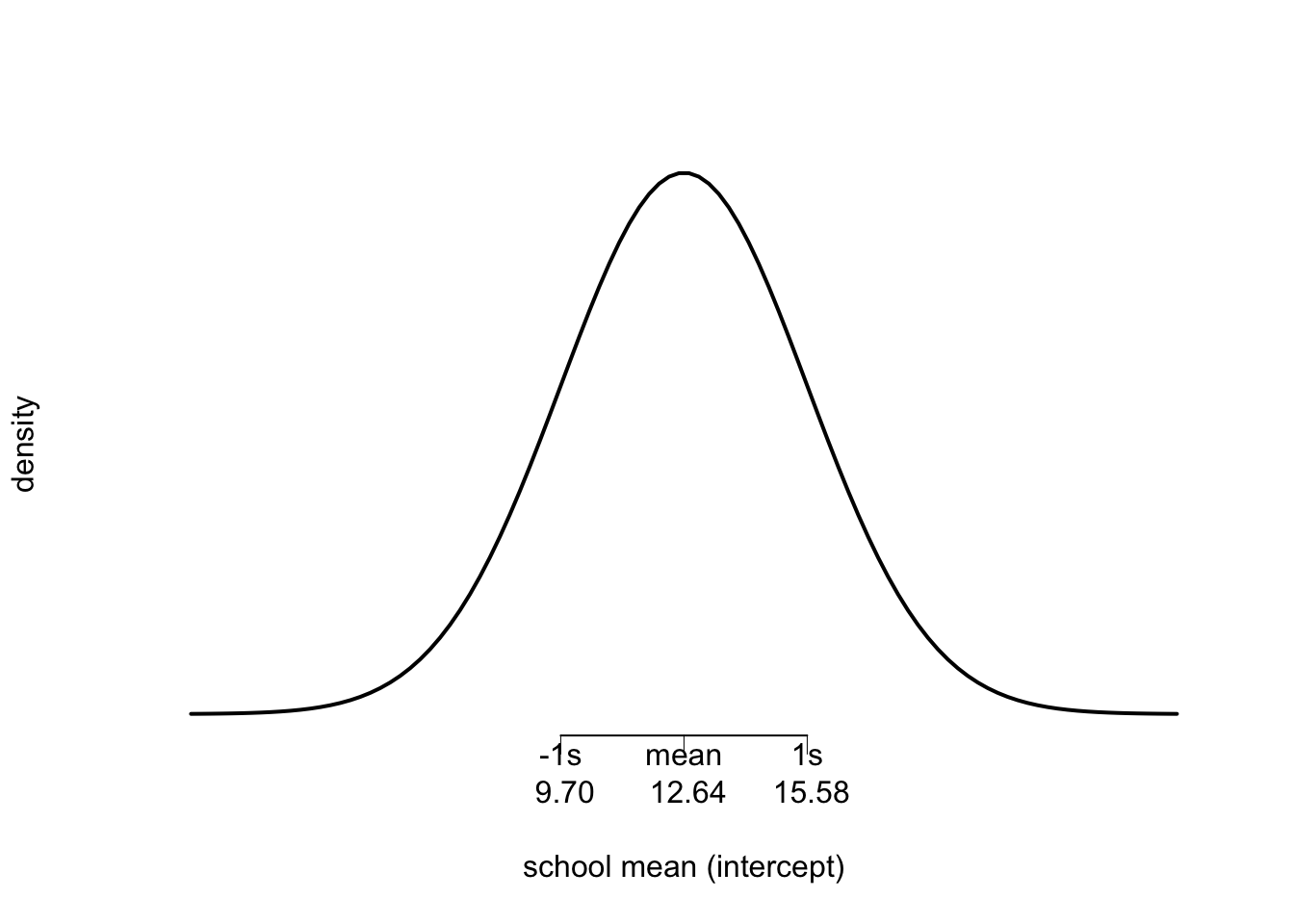
We’ll also discuss the assumption of normality of the random effects next week. The intercept and standard deviation of the random effects together give us information about the unconditional distribution of mean math scores:

\(\hat{\mu}_{..} = 12.64\), \(95\% \text{ CI } (12.16, 13.14)\) \(\text{SD} = 2.94\), \(95\% \text{ CI } (2.55, 3.26)\)

We can see in the plot below, that theoretically, most (\(\sim 68 \%\)) of the schools have mean math achievement between \(\sim 9.70\) and \(\sim 15.50\)

6.6 Linear mixed-effects

For illustration, we’ll fit a model where a student’s math achievement is a function of their group-centered SES (cses). We’ll learn some different terminology for this in the next two weeks, but here, we’re going to contrast the fixed-effect estimate from lmer with that from lm.

Here’s how we include a predictor in lmer:

mod2_re <- lmer(mathach ~ cses + (1|school), data = HSB)
summary(mod2_re)

## Linear mixed model fit by REML ['lmerMod']
## Formula: mathach ~ cses + (1 | school)
##    Data: HSB
## 
## REML criterion at convergence: 46724
## 
## Scaled residuals: 
##     Min      1Q  Median      3Q     Max 
## -3.0969 -0.7322  0.0194  0.7572  2.9147 
## 
## Random effects:
##  Groups   Name        Variance Std.Dev.
##  school   (Intercept)  8.672   2.945   
##  Residual             37.010   6.084   
## Number of obs: 7185, groups:  school, 160
## 
## Fixed effects:
##             Estimate Std. Error t value
## (Intercept)  12.6361     0.2445   51.68
## cses          2.1912     0.1087   20.17
## 
## Correlation of Fixed Effects:
##      (Intr)
## cses 0.000

Now, with lm() we ignore the fact that students are grouped

mod2_lm <- lm(mathach ~ cses, data = HSB)
summary(mod2_lm)

## 
## Call:
## lm(formula = mathach ~ cses, data = HSB)
## 
## Residuals:
##      Min       1Q   Median       3Q      Max 
## -17.8660  -5.1165   0.2966   5.3880  14.8705 
## 
## Coefficients:
##             Estimate Std. Error t value Pr(>|t|)    
## (Intercept) 12.74785    0.07933  160.69   <2e-16 ***
## cses         2.19117    0.12010   18.24   <2e-16 ***
## ---
## Signif. codes:  0 '***' 0.001 '**' 0.01 '*' 0.05 '.' 0.1 ' ' 1
## 
## Residual standard error: 6.725 on 7183 degrees of freedom
## Multiple R-squared:  0.04429,    Adjusted R-squared:  0.04415 
## F-statistic: 332.8 on 1 and 7183 DF,  p-value: < 2.2e-16

Note that the cses effects are similar, but with different standard errors, and that the intercept estimate is essentially the sample average math achievement in lm, ignoring the grouping by school. We also do not get any information about variability in the school means.

6.6.1 Random effects estimates

Let’s go back to the first model and see some of the random effects estimates:

ran <- ranef(mod1_re)
ran$school$`(Intercept)`[1:10]

##  [1] -2.6639348  0.7394098 -4.5684656  2.9485171  0.4939461 -1.2425116 -2.5023497  6.2682432  4.9621083
## [10]  3.6965749

These are simply the amount by which school \(J\) deviates from the estimated mean of \(12.64\).

We can also get the estimated school means. Note, these are NOT the actual means of the scores within each school. In later weeks, we’ll discuss that these are Empirical Bayes estimates, which are shrinkage estimates. When a school’s mean is not precisely captured in the sample, the estimate shrinks toward the grand mean (\(12.64\)). When a school’s estimate is precise, the estimated mean is less influenced by the grand mean.

In this way, estimates of smaller or less precisely estimated schools take information from the rest of the distribution.

cof <- coef(mod1_re)
cof$school$`(Intercept)`[1:10]

##  [1]  9.973039 13.376384  8.068508 15.585491 13.130920 11.394462 10.134624 18.905217 17.599082
## [10] 16.333549

As we see, the estimated mean math achievement in school 1308 is \(15.59\) while the actual sample average is:

mean(HSB$mathach[HSB$school == "1308"])

## [1] 16.2555

Summary:

1. We have now started to use lmer the main function for fitting mixed-effects models with REML (and with ML)
2. We’ve seen some simple output and computed the intraclass correlation
3. We’ve discussed a bit about the distribution of random effects and their estimates

Next week, we’ll pull this together in the context of an actual research question.